D2L 学习简记

电子书：动手学深度学习

1. 引言

介绍了常见的机器学习问题，了解即可。

2. 预备知识

简单介绍了 PyTorch 包最底层的一些操作，感觉没必要细看，需要用的时候再查即可。

3. 线性神经网络

3.1 线性回归

线性问题模型

设特征向量为, 权重向量为, 偏置项为, 则线性神经网络的输出为：

对于特征集合, 预测值可通过矩阵-向量乘法表示为：

损失函数

在用模型拟合（fit）数据之前，我们需要损失函数（loss function）来量化实际值和预测值的差距。

设样本的预测值为，其相应的真实标签为。

平方误差

均方误差 (Mean Squared Error, MSE)：

平均绝对误差（Mean Absolute Error, MAE）：

Huber Loss

接下来的讨论都基于 MSE 损失函数。

目标

给定训练数据特征和对应的已知标签，线性回归的目标是找到一组权重向量和偏置：当给定从的同分布中取样的新样本特征时，这组权重向量和偏置能够使得新样本预测标签的误差尽可能小。

即，我们希望找到一组参数。

解析解

线性回归的解可用一个公式简答表达出来，这类解被称为解析解（analytical solution）。

线性回归的解析解为：

解析解对问题的限制很严格，只有像线性回归这样的简单问题存在解析解。因此它无法被广泛应用于深度学习里。

随机梯度下降（Stochastic Gradient Descent, SGD）

梯度下降法通过不断地在损失函数递减的方向上更新参数来降低误差，这种方法几乎可以优化所有深度学习模型。

遍历整个训练数据集效率太低，因此通常采用小批量随机梯度下降（mini-batch SGD）来降低计算量。

在每次迭代中，首先随机抽样一个小批量，它是由固定数量的训练样本组成的。然后计算的平均损失关于模型参数的导数（即梯度）。最后，将梯度乘以一个预先确定的正数，并从当前参数的值中减掉。

数学公式看起来比较直观：

训练步骤

初始化模型参数的值，如随机初始化；
- 从数据集中随机抽取小批量样本且在负梯度的方向上更新参数，并不断迭代这一步骤。对于平方损失和仿射变换，可以明确地写成如下形式：
- 称为批量大小（batch size），为学习率（learning rate）。这两个值通常是预先指定而非模型训练得到的。称这些可以调整但不在训练过程中更新的参数称为超参数（hyperparameter），调整他们的过程为调参（hyperparameter tuning）。
- 超参数通常根据训练迭代结果调整，而训练迭代结果是在独立的验证数据集（validation dataset）上评估得到的。
在训练了预先确定的若干迭代次数（epoch）后，就得到了模型参数的估计值和。不过，即使我们的函数确实是线性的且无噪声，这些估计值也不会使损失函数真正地达到最小值。因为算法会使得损失向最小值缓慢收敛，但却不能在有限的步数内非常精确地达到最小值。

模型预测

给定特征估计目标的过程通常称为预测（prediction）或推断（inference）。前者在语义上似乎更得当。

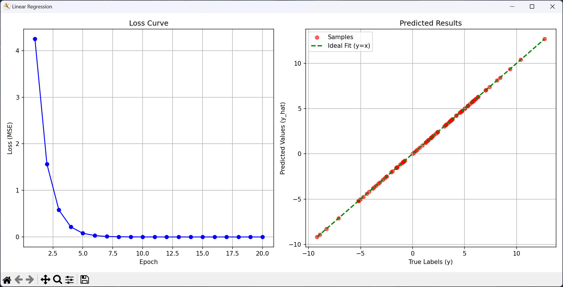
3.2 线性回归代码实现

Talk is cheap, show me the code?

import torch
from torch import Tensor
import random
from matplotlib import pyplot as plt
from typing import Tuple, Generator, Any

def generator(true_w: Tensor, true_b: float, size: int = 2000) -> tuple[Tensor, Tensor]:
    """线性模型加噪声构造数据集"""
    X = torch.normal(0, 1, (size, len(true_w)))
    y = X @ true_w + true_b
    # 加上高斯噪声
    y += torch.normal(0, 0.01, y.shape)
    return X, y.reshape(-1, 1)

def data_iter(batch_size: int, features: Tensor, labels: Tensor) -> Generator[Tuple, Any, None]:
    """随机读取小批量数据的数据迭代器"""
    examples = len(features)
    indices = list(range(examples))
    random.shuffle(indices)
    for i in range(0, examples, batch_size):
        batch_indices = torch.tensor(indices[i: min(i + batch_size, examples)])
        yield features[batch_indices], labels[batch_indices]

def linreg(X: Tensor, w: Tensor, b: Tensor):
    """线性回归模型"""
    return X @ w + b

def squared_loss(y_hat: Tensor, y: Tensor):
    """均方损失"""
    return (y_hat - y.reshape(y_hat.shape)) ** 2 / 2

def sgd(params: list[Tensor], lr: float, batch_size: int):
    """小批量随机梯度下降"""
    with torch.no_grad():
        for param in params:
            param -= lr * param.grad / batch_size
            param.grad.zero_()

def train():
    """训练模型"""
    # 真实模型以及数据集
    true_w = torch.tensor([1.1, -4.5, 1.4])
    true_b = 1.1919810
    features, labels = generator(true_w, true_b)

    # 超参数
    batch_size = 30
    lr = 0.008
    epochs = 20

    # 模型初始化
    net = linreg
    loss = squared_loss
    w = torch.normal(0, 0.01, size = (3, 1), requires_grad = True)
    b = torch.zeros(1, requires_grad = True)

    loss_history = []
    for epoch in range(1, epochs + 1):
        for X, y in data_iter(batch_size, features, labels):
            # 1. 正向传播：计算预测值
            l = loss(net(X, w, b), y)

            # 2. 反向传播：计算梯度
            # l 是一个形状为 (batch_size, 1) 的向量，sum() 后变为标量才能 backward
            l.sum().backward()

            #3. 参数更新
            sgd([w, b], lr, batch_size)

        # 每个 epoch 打印一次训练误差
        with torch.no_grad():
            train_l = loss(net(features, w, b), labels)
            l = float(train_l.mean())
            loss_history.append(l)
            print(f"epoch {epoch}, loss {l:f}")
    
    print("-" * 30)
    print(f"Δw: {true_w - w.reshape(true_w.shape)}")
    print(f"Δb: {true_b - b}")

    # 可视化结果
    plt.figure(figsize = (13, 6))
    plt.gcf().canvas.manager.set_window_title("Linear Regression")
    
    # loss 曲线
    plt.subplot(1, 2, 1)
    plt.plot(range(1, epochs + 1), loss_history, marker = "o", color = "b")
    plt.xlabel("Epoch")
    plt.ylabel("Loss (MSE)")
    plt.title("Loss Curve")
    plt.grid(True)

    # 预测值和真实值在对角线上的散点图
    # 随 100 个点
    with torch.no_grad():
        sample_idx = torch.randperm(len(features))[:100]
        sample_features = features[sample_idx]
        sample_labels = labels[sample_idx]
        predictions = net(sample_features, w, b)

    plt.subplot(1, 2, 2)
    plt.scatter(sample_labels.numpy(), predictions.numpy(), alpha = 0.6, color = "red", label = "Samples")

    min_val = min(sample_labels.min(), predictions.min())
    max_val = max(sample_labels.max(), predictions.max())
    plt.plot([min_val, max_val], [min_val, max_val], 'g--', linewidth = 2, label = "Ideal Fit (y=x)")

    plt.xlabel("True Labels (y)")
    plt.ylabel("Predicted Values (y_hat)")
    plt.title("Predicted Results")
    plt.legend()
    plt.grid(True)

    plt.tight_layout()
    plt.show()

if __name__ == "__main__":
    train()

当然也可以用 PyTorch 的高级 API 来实现线性回归，这里就不搓了。

3.3 softmax 回归

softmax 回归用于解决多分类问题，其输出是一个概率分布。（本质是把全连接层的输出序列变成一个概率序列）

~~为什么不直接叫 softmax 分类呢？~~

和线性回归一样，softmax 回归也是一个单层神经网络，其输出层也是一个全连接层（fully‐connected layer）。

个输入，个输出的全连接层，参数开销为。将个输入转化为个输出的成本可减少到，其中超参数可灵活指定，平衡参数节约和模型有效性。

分类问题模型

数据分类可使用 独热编码（one-hot encoding）。

我们需要根据输入，给出每个分类的概率。

softmax 运算

我们希望模型的输出可以视为属于类的概率，然后选择具有最大输出值的类别作为我们的预测。

我们无法将线性层的输出向量直接视为概率，因为其不一定符合概率的非负性和归一性。这时就需要神奇的 softmax 函数了：

$其中$

容易验证，可视为一个正确的概率分布，且不会改变未规范预测化的之间的大小关系，于是有：

尽管 softmax 是一个非线性函数，但 softmax 回归的输出仍然由输入特征的仿射变换决定，因此，softmax 回归是一个线性模型（linear model）。

softmax 运算可通过小批量样本的矢量化来加速。设特征维度（输入数列）为，批量大小为，输出类别数为，并有小批量样本的特征，权重，偏置，则 softmax 回归的矢量计算表达式为：

交叉熵损失

分类任务的基石，源于信息论，用于衡量两个概率分布之间的差异。

对于任何标签和模型预测，定义交叉熵损失函数为：

特别地，相对于任何未规范化的预测，其导数为：

推导过程先咕了。

3.4 softmax 回归实现 Fashion-MNIST 分类

就算知道是怎么一回事，实现起来也还是有点难度的。

import time
import torch
import torchvision
from torch import Tensor
from torchvision import transforms
from matplotlib import pyplot as plt

# 设置超参数
BATCH_SIZE = 256
LEARNING_RATE = 0.1
EPOCHS = 30
DEVICE = torch.device("cuda" if torch.cuda.is_available() else "cpu")
print(f"Device: {DEVICE}")
print(f"Batch Size: {BATCH_SIZE}")
print(f"Learning Rate: {LEARNING_RATE}")

# 加载数据集
train_data = torchvision.datasets.FashionMNIST(root = './fashion_mnist', train = True, transform = transforms.ToTensor(), download = True)
test_data = torchvision.datasets.FashionMNIST(root = './fashion_mnist', train = False, transform = transforms.ToTensor(), download = True)

train_loader = torch.utils.data.DataLoader(train_data, batch_size = BATCH_SIZE, shuffle = True)
test_loader = torch.utils.data.DataLoader(test_data, batch_size = BATCH_SIZE, shuffle = False)

# 初始化模型参数
N_INPUT = 784
N_OUTPUT = 10

W = torch.normal(0, 0.01, size = (N_INPUT, N_OUTPUT), device = DEVICE, requires_grad = True)
b = torch.zeros(N_OUTPUT, device = DEVICE, requires_grad = True)

def softmax(X: Tensor) -> Tensor:
    """计算 softmax 值"""
    X_exp = torch.exp(X)
    partition = X_exp.sum(dim = 1, keepdim = True)
    return X_exp / partition
    # 注意，这里没有防止数值溢出

def net(X: Tensor) -> Tensor:
    """输入特征 X，返回模型预测输出"""
    return softmax(X.reshape((-1, W.shape[0])) @ W + b)

def cross_entropy(y_hat: Tensor, y: Tensor) -> Tensor:
    """交叉熵损失"""
    return - torch.log(y_hat[range(len(y_hat)), y])

def accuracy(y_hat: Tensor, y: Tensor) -> float:
    """计算精度"""
    if len(y_hat.shape) > 1 and y_hat.shape[1] > 1:
        y_hat = y_hat.argmax(axis = 1)
    cmp = y_hat.type(y.dtype) == y
    return float(cmp.type(y.dtype).sum())

def sgd(params: list[Tensor], lr: float, batch_size: int):
    """小批量随机梯度下降"""
    with torch.no_grad():
        for param in params:
            param -= lr * param.grad / batch_size
            param.grad.zero_()

def train():
    """训练模型"""
    loss_history = []
    acc_history = []

    print(f"{'=' * 15} Training Process {'=' * 15}")
    stime = time.time()

    for epoch in range(1, EPOCHS + 1):
        metric = [0.0, 0.0, 0.0] # 训练损失总和，训练准确度总和，样本数

        for X, y in train_loader:
            # 将数据移动到设备
            X, y = X.to(DEVICE), y.to(DEVICE)

            # 正向传播
            y_hat = net(X)
            l = cross_entropy(y_hat, y)

            # 反向传播
            l.sum().backward()

            # 参数更新
            sgd([W, b], LEARNING_RATE, BATCH_SIZE)

            # 记录指标
            with torch.no_grad():
                metric[0] += l.sum().item()
                metric[1] += accuracy(y_hat, y)
                metric[2] += X.shape[0]

        loss_history.append(metric[0] / metric[2])
        acc_history.append(metric[1] / metric[2])
        
        print(f"Epoch {epoch}/{EPOCHS}, Loss: {loss_history[-1]:.4f}, Accuracy: {acc_history[-1]:.4f}")

    etime = time.time()
    print(f"{'=' * 15} Time Usage: {etime - stime:.0f}s {'=' * 15}")

    # 在测试集上评估
    acc_sum, n = 0.0, 0
    with torch.no_grad():
        for X, y in test_loader:
            X, y = X.to(DEVICE), y.to(DEVICE)
            acc_sum += accuracy(net(X), y)
            n += y.numel()

    print(f"\nTest Accuracy: {acc_sum / n:.4f}")

    # 绘制 Loss 和 Accuracy 曲线
    plt.figure(figsize = (10, 5))
    plt.gcf().canvas.manager.set_window_title("Softmax Regression")

    # Loss
    plt.subplot(1, 2, 1)
    plt.plot(range(1, EPOCHS + 1), loss_history, label = "Train Loss", color = "red")
    plt.xlabel("Epochs")
    plt.ylabel("Loss")
    plt.title("Loss Curve")
    plt.legend()
    plt.grid(True)

    # Accuracy
    plt.subplot(1, 2, 2)
    plt.plot(range(1, EPOCHS + 1), acc_history, label = "Train Accuracy", color = "green")
    plt.xlabel("Epochs")
    plt.ylabel("Accuracy")
    plt.title("Accuracy Curve")
    plt.legend()
    plt.grid(True)

    plt.tight_layout()
    plt.show()

if __name__ == "__main__":
    train()

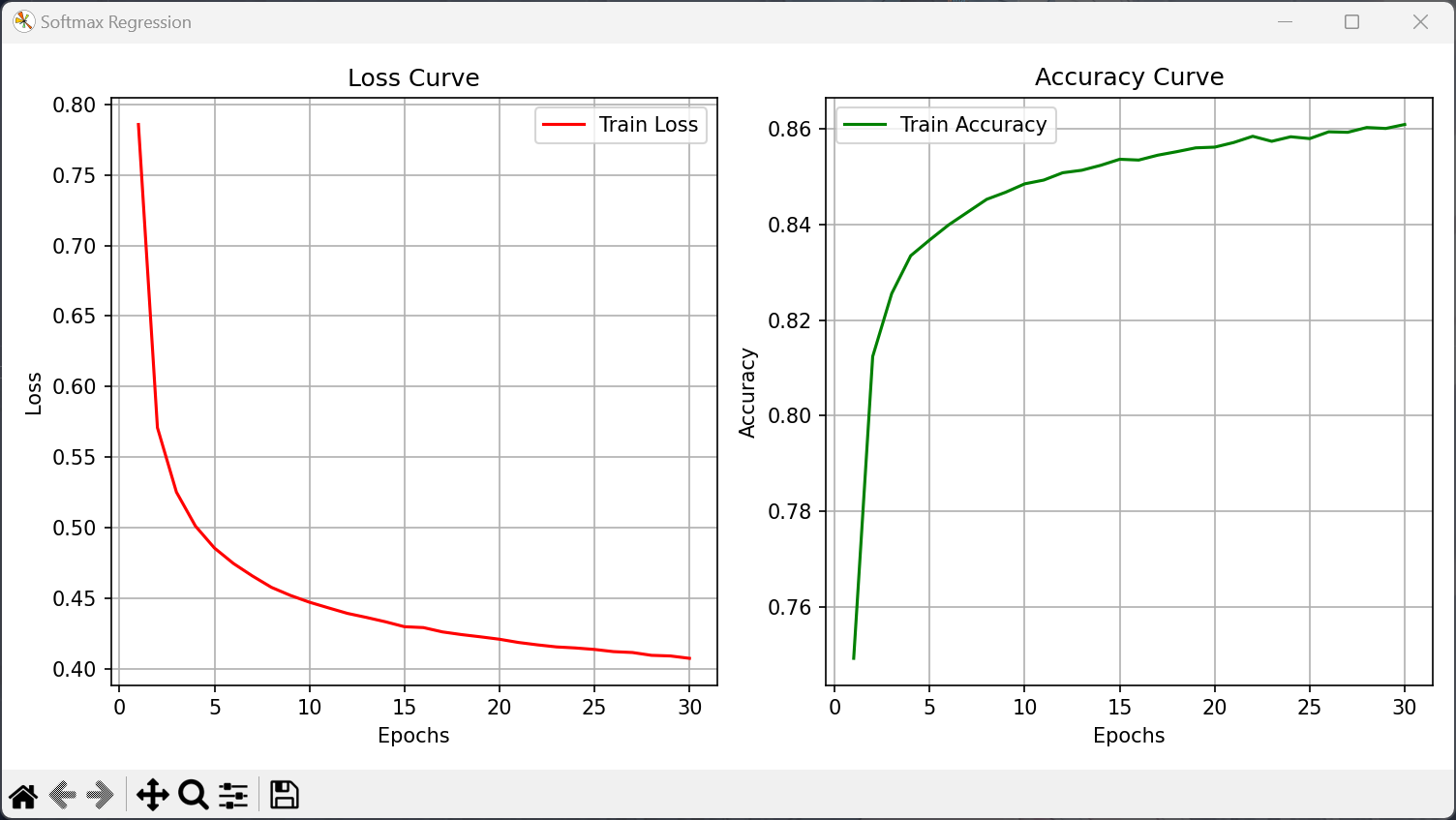
训练输出：

Device: cuda
Batch Size: 256
Learning Rate: 0.1
=============== Training Process ===============
Epoch 1/30, Loss: 0.7859, Accuracy: 0.7493
...
Epoch 30/30, Loss: 0.4072, Accuracy: 0.8609
=============== Time Usage: 145s ===============

Test Accuracy: 0.8417

4. 多层感知机

线性模型假设特征与输出之间存在线性关系，这种假设在许多实际问题中是不成立的。

为了处理更普遍的函数关系类型，我们需要非线性变换，这可以通过堆层、引入非线性激活函数等来实现。

4.1 隐藏层

在输入层与输出层之间的层，称为隐藏层（hidden layer）。

我们可以通过在网络中加入一个或多个隐藏层来克服线性模型的限制，使其能处理更普遍的函数关系类型。

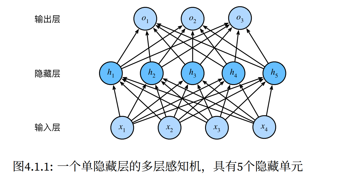
要做到这一点，最简单的方法是将许多全连接层堆叠在一起。每一层都输出到上面的层，直到生成最后的输出。我们可以把前层看作表示，把最后一层看作线性预测器。这种架构通常称为多层感知机（Multilayer Perceptron, MLP）。

如下如所示（图片截自 D2L）：

不过，具有全连接层的多层感知机的参数开销可能会爆炸，需要合理地设置隐藏层的大小。

4.2 激活函数

隐藏单元由输入的仿射函数给出，输出只是隐藏单元的仿射函数。仿射函数的仿射函数本身就是仿射函数，而之前的线性模型已经能够表示任何仿射函数。

为了防止多层感知机退化成线性模型，需要引入非线性的激活函数。

常见的激活函数有 Sigmoid、tanh、ReLU、Leaky ReLU 等，这里就不一一展开介绍了。

4.3 实现 MLP

这里做一个双隐藏层的简单 MLP，激活函数用 ReLU。

只要在之前的 softmax 回归的代码基础上稍作修改即可。

import time
import torch
import torchvision
from torch import Tensor
from torchvision import transforms
from matplotlib import pyplot as plt

# 设置超参数
BATCH_SIZE = 256
LEARNING_RATE = 0.1
EPOCHS = 30
DEVICE = torch.device("cuda" if torch.cuda.is_available() else "cpu")
print(f"Device: {DEVICE}")
print(f"Batch Size: {BATCH_SIZE}")
print(f"Learning Rate: {LEARNING_RATE}")

# 加载数据集
train_data = torchvision.datasets.FashionMNIST(root = './fashion_mnist', train = True, transform = transforms.ToTensor(), download = True)
test_data = torchvision.datasets.FashionMNIST(root = './fashion_mnist', train = False, transform = transforms.ToTensor(), download = True)

train_loader = torch.utils.data.DataLoader(train_data, batch_size = BATCH_SIZE, shuffle = True)
test_loader = torch.utils.data.DataLoader(test_data, batch_size = BATCH_SIZE, shuffle = False)

# 初始化模型参数
N_INPUT = 784
N_HIDDEN_1 = 256  # 第一个隐藏层的神经元数量
N_HIDDEN_2 = 128  # 第二个隐藏层的神经元数量
N_OUTPUT = 10

# 第一层：输入 -> 隐藏层1
W1 = torch.normal(0, 0.01, size = (N_INPUT, N_HIDDEN_1), device = DEVICE, requires_grad = True)
b1 = torch.zeros(N_HIDDEN_1, device = DEVICE, requires_grad = True)

# 第二层：隐藏层1 -> 隐藏层2
W2 = torch.normal(0, 0.01, size = (N_HIDDEN_1, N_HIDDEN_2), device = DEVICE, requires_grad = True)
b2 = torch.zeros(N_HIDDEN_2, device = DEVICE, requires_grad = True)

# 第三层：隐藏层2 -> 输出
W3 = torch.normal(0, 0.01, size = (N_HIDDEN_2, N_OUTPUT), device = DEVICE, requires_grad = True)
b3 = torch.zeros(N_OUTPUT, device = DEVICE, requires_grad = True)

params = [W1, b1, W2, b2, W3, b3]

def relu(X: Tensor) -> Tensor:
    a = torch.zeros_like(X)
    return torch.max(X, a)

def softmax(X: Tensor) -> Tensor:
    """计算 softmax 值"""
    X_exp = torch.exp(X)
    partition = X_exp.sum(dim = 1, keepdim = True)
    return X_exp / partition
    # 注意，这里没有防止数值溢出

def net(X: Tensor) -> Tensor:
    """输入特征 X，经过两层隐藏层后返回预测输出"""
    # 展平输入：(Batch, 1, 28, 28) -> (Batch, 784)
    X = X.reshape((-1, N_INPUT))
    
    # 第一层
    H1 = relu(X @ W1 + b1)
    # 第二层
    H2 = relu(H1 @ W2 + b2)
    # 输出层
    return softmax(H2 @ W3 + b3)

def cross_entropy(y_hat: Tensor, y: Tensor) -> Tensor:
    """交叉熵损失"""
    return - torch.log(y_hat[range(len(y_hat)), y])

def accuracy(y_hat: Tensor, y: Tensor) -> float:
    """计算精度"""
    if len(y_hat.shape) > 1 and y_hat.shape[1] > 1:
        y_hat = y_hat.argmax(axis = 1)
    cmp = y_hat.type(y.dtype) == y
    return float(cmp.type(y.dtype).sum())

def sgd(params: list[Tensor], lr: float, batch_size: int):
    """小批量随机梯度下降"""
    with torch.no_grad():
        for param in params:
            param -= lr * param.grad / batch_size
            param.grad.zero_()

def train():
    """训练模型"""
    loss_history = []
    acc_history = []

    print(f"{'=' * 15} Training Process {'=' * 15}")
    stime = time.time()

    for epoch in range(1, EPOCHS + 1):
        metric = [0.0, 0.0, 0.0] # 训练损失总和，训练准确度总和，样本数

        for X, y in train_loader:
            # 将数据移动到设备
            X, y = X.to(DEVICE), y.to(DEVICE)

            # 正向传播
            y_hat = net(X)
            l = cross_entropy(y_hat, y)

            # 反向传播
            l.sum().backward()

            # 参数更新
            sgd(params, LEARNING_RATE, BATCH_SIZE)

            # 记录指标
            with torch.no_grad():
                metric[0] += l.sum().item()
                metric[1] += accuracy(y_hat, y)
                metric[2] += X.shape[0]

        loss_history.append(metric[0] / metric[2])
        acc_history.append(metric[1] / metric[2])
        
        print(f"Epoch {epoch}/{EPOCHS}, Loss: {loss_history[-1]:.4f}, Accuracy: {acc_history[-1]:.4f}")

    etime = time.time()
    print(f"{'=' * 15} Time Usage: {etime - stime:.0f}s {'=' * 15}")

    # 在测试集上评估
    acc_sum, n = 0.0, 0
    with torch.no_grad():
        for X, y in test_loader:
            X, y = X.to(DEVICE), y.to(DEVICE)
            acc_sum += accuracy(net(X), y)
            n += y.numel()

    print(f"\nTest Accuracy: {acc_sum / n:.4f}")

    # 绘制 Loss 和 Accuracy 曲线
    plt.figure(figsize = (10, 5))
    plt.gcf().canvas.manager.set_window_title("Simple MLP")

    # Loss
    plt.subplot(1, 2, 1)
    plt.plot(range(1, EPOCHS + 1), loss_history, label = "Train Loss", color = "red")
    plt.xlabel("Epochs")
    plt.ylabel("Loss")
    plt.title("Loss Curve")
    plt.legend()
    plt.grid(True)

    # Accuracy
    plt.subplot(1, 2, 2)
    plt.plot(range(1, EPOCHS + 1), acc_history, label = "Train Accuracy", color = "green")
    plt.xlabel("Epochs")
    plt.ylabel("Accuracy")
    plt.title("Accuracy Curve")
    plt.legend()
    plt.grid(True)

    plt.tight_layout()
    plt.show()

if __name__ == "__main__":
    train()

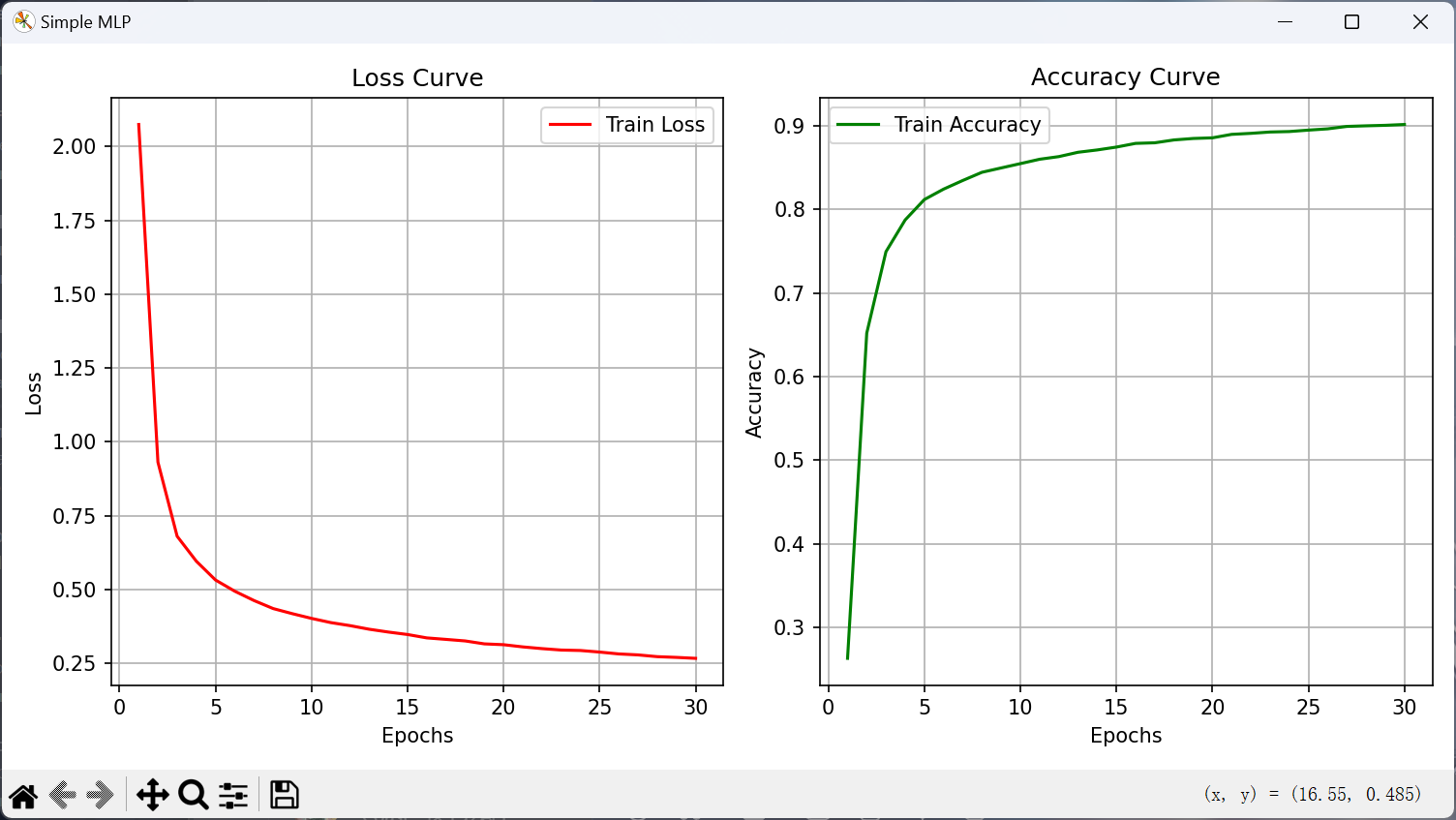
训练输出：

Device: cuda
Batch Size: 256
Learning Rate: 0.1
=============== Training Process ===============
Epoch 1/30, Loss: 2.0744, Accuracy: 0.2627
...
Epoch 30/30, Loss: 0.2668, Accuracy: 0.9015
=============== Time Usage: 156s ===============

Test Accuracy: 0.8786

表现略好于之前的 softmax 回归。

4.4 咕咕本章其它部分

此后，该书插入讲解了模型选择、欠拟合和过拟合、正则化、权重衰减、Dropout等内容，这些内容比较零碎，感觉没必要特地记录，故先略过。

5. 深度学习计算

5.1 层和块

为了实现复杂的网络，需引入神经网络块的概念。块 (block) 可以描述单个层、由多个层组成的组件或整个模型本身。使用块进行抽象的一个好处就是组合方便、代码实现简洁。

很自然地，在代码编写中，可以用类来表示块。这个类的任何子类需要包含：

任何必需的参数（parameters）；
将输入转为输出的前向传播函数（forward）；
用于计算梯度的反向传播函数（backward）。

在定义我们自己的块时，由于自动微分提供了一些后端实现，我们只需要考虑前向传播函数和必需的参数。

5.2 重构 MLP

现在，应用层和块的思想，并使用 PyTorch 的高级 API 来重构原来的丑陋 MPL。

具体来说：

使用 torch.optim.AdamW 优化器替换 sgd 函数。
使用 nn.Sequential 替换 net 函数。
使用 nn.Linear 层自动管理权重 W 和偏置 b。
使用 nn.CrossEntropyLoss 来计算交叉熵损失。
使用 model.train() 与 model.eval() 来切换训练和测试模式。

比原来优雅多了。

import time
import torch
import torchvision
from torch import Tensor
from torch import nn
from torchvision import transforms
from matplotlib import pyplot as plt

# 设置超参数
BATCH_SIZE = 256
LEARNING_RATE = 0.001   # AdamW 的默认学习率
EPOCHS = 30
DEVICE = torch.device("cuda" if torch.cuda.is_available() else "cpu")
print(f"Device: {DEVICE}")
print(f"Batch Size: {BATCH_SIZE}")
print(f"Learning Rate: {LEARNING_RATE}")

# 加载数据集
train_data = torchvision.datasets.FashionMNIST(root = './fashion_mnist', train = True, transform = transforms.ToTensor(), download = True)
test_data = torchvision.datasets.FashionMNIST(root = './fashion_mnist', train = False, transform = transforms.ToTensor(), download = True)

train_loader = torch.utils.data.DataLoader(train_data, batch_size = BATCH_SIZE, shuffle = True)
test_loader = torch.utils.data.DataLoader(test_data, batch_size = BATCH_SIZE, shuffle = False)

# 定义模型类
class MLP(nn.Module):
    def __init__(self, input_size, hidden_1, hidden_2, output_size):
        super(MLP, self).__init__()
        # nn.Sequential 是一个容器，数据会按顺序通过这些层
        self.net = nn.Sequential(
            nn.Flatten(),
            nn.Linear(input_size, hidden_1),
            nn.ReLU(),
            nn.Linear(hidden_1, hidden_2),
            nn.ReLU(),
            nn.Linear(hidden_2, output_size)
        )

    def forward(self, x):
        return self.net(x)

# 初始化模型参数
N_INPUT = 784
N_HIDDEN_1 = 256  # 第一个隐藏层的神经元数量
N_HIDDEN_2 = 128  # 第二个隐藏层的神经元数量
N_OUTPUT = 10

model = MLP(N_INPUT, N_HIDDEN_1, N_HIDDEN_2, N_OUTPUT).to(DEVICE)

loss_fn = nn.CrossEntropyLoss()
optimizer = torch.optim.AdamW(model.parameters(), lr = LEARNING_RATE)

def accuracy(y_hat: Tensor, y: Tensor) -> float:
    """计算精度"""
    pred = y_hat.argmax(dim = 1)
    correct = (pred == y).sum().item()
    return correct

def evaluate(model, data_loader):
    """在测试集上评估模型"""
    model.eval()
    acc_sum, n = 0.0, 0
    with torch.no_grad():
        for X, y in data_loader:
            X, y = X.to(DEVICE), y.to(DEVICE)
            y_hat = model(X)
            acc_sum += accuracy(y_hat, y)
            n += y.size(0)
    return acc_sum / n

def train():
    """训练模型"""
    loss_history = []
    acc_history = []

    print(f"{'=' * 15} Training Process {'=' * 15}")
    stime = time.time()

    for epoch in range(1, EPOCHS + 1):
        model.train()
        loss_sum = 0.0
        correct_sum = 0
        tot = 0

        for X, y in train_loader:
            X, y = X.to(DEVICE), y.to(DEVICE)
            # 前向传播
            y_hat = model(X)
            loss = loss_fn(y_hat, y)
            # 梯度清零
            optimizer.zero_grad()
            # 反向传播
            loss.backward()
            # 参数更新
            optimizer.step()
            # 记录统计信息
            batch_size = y.size(0)
            loss_sum += loss.item() * batch_size
            correct_sum += accuracy(y_hat, y)
            tot += batch_size
        loss_history.append(loss_sum / tot)
        acc_history.append(correct_sum / tot)
        print(f"Epoch {epoch}/{EPOCHS}, Loss: {loss_history[-1]:.4f}, Accuracy: {acc_history[-1]:.4f}")

    test_acc = evaluate(model, test_loader)
    print(f"\nTest Accuracy: {test_acc:.4f}")

    # 绘制 Loss 和 Accuracy 曲线
    plt.figure(figsize = (10, 5))
    plt.gcf().canvas.manager.set_window_title("Simple MLP")

    # Loss
    plt.subplot(1, 2, 1)
    plt.plot(range(1, EPOCHS + 1), loss_history, label = "Train Loss", color = "red")
    plt.xlabel("Epochs")
    plt.ylabel("Loss")
    plt.title("Loss Curve")
    plt.legend()
    plt.grid(True)

    # Accuracy
    plt.subplot(1, 2, 2)
    plt.plot(range(1, EPOCHS + 1), acc_history, label = "Train Accuracy", color = "green")
    plt.xlabel("Epochs")
    plt.ylabel("Accuracy")
    plt.title("Accuracy Curve")
    plt.legend()
    plt.grid(True)

    plt.tight_layout()
    plt.show()

if __name__ == "__main__":
    train()

5.3 save & load

SL Tensor

令 x : Tensor。

Save

调用 torch.save。

torch.save(x, "x-file")

Load

调用 torch.load。

x = torch.load("x-file")

SL Model

令 model : nn.Module。

Save

一般来说，我们只需要保存模型的参数，而不需要保存模型的结构。

调用 model.state_dict() 得到模型参数字典。
调用 torch.save 保存参数字典。

torch.save(model.state_dict(), "model.params")

Load

调用 model.load_state_dict。

model = Model() # 先实例化一个模型类
model.load_state_dict(torch.load("model.params"))

SL Optimizer

令 optimizer : torch.optim.Optimizer。

Save

一般来说，我们只需要保存优化器的参数，而不需要保存优化器的结构。

调用 optimizer.state_dict() 得到优化器参数字典。
调用 torch.save 保存参数字典。

torch.save(optimizer.state_dict(), "optimizer.params")

Load

调用 optimizer.load_state_dict。

optimizer = Optimizer() # 先实例化一个优化器类
optimizer.load_state_dict(torch.load("optimizer.params"))

5.4 咕咕本章其它部分

该书还介绍了参数管理、延后初始化、自定义层、设置计算设备等不太需要记录的内容，直接略过。

6. 卷积神经网络

多层感知机无法处理高维感知数据。全连接层的参数量会爆炸，且隐藏层不足以学习到良好的特征。

卷积神经网络（Convolutional Neural Networks，CNN）是解决这种问题的一种创造性方法。

6.1 从全连接到卷积

卷积层

设多层感知机的输入为二维图像，其隐藏表示为同大小的二维张量，再分别用与表示位置的元素。为了让每个隐藏单元都接收到每个像素的信息（没错，非常浪费），设参数为四阶权重张量。再假设二阶张量包含了偏置，于是就有：

$其中$

简单来说，就是可以直接用偏移来重新索引。对于隐藏表示中的，可以通过在中以为中心对像素进行加权求和而得，加权所用权重为。

考虑以下两个有用的性质：

平移不变性（translation invariance）：不管检测对象出现在输入的哪个位置，神经网络的前几层应该对相同的区域有相似的反应。这意味着检测对象在输入中的平移，应该仅导致隐藏表示中的平移。
局部性（locality）：神经网络的每一层都应该只学习到局部特征，而不过度在意相隔较远区域的信息，最后再通过聚合局部特征预测整体特征。这意味着隐藏表示应该与输入的局部邻域相关。

由平移不变性，与与无关，因此即为一常数，可记为二维张量，于是的表示可被极大地简化：

这个式子就是互相关运算（cross‐correlation）.

再考虑局部性，我们不应过度考虑偏离太远的地方。于是干脆一点，当或时，就为零。于是的表示可重写为：

上式即为一个卷积层（convolutional layer），其中称为卷积核（convolution kernel）或滤波器（filter）。

相比全连接层，卷积层极大减少了参数量，需要注意的是，仅当输入具有平移不变性时，才能使用卷积表示！

通道

上面提到的卷积层的输入是二维图像，但实际应用中，图像一般包含了三个通道（三种原色，如 RGB）。因此图像实际上是三维张量，除了前面的两个空间维度外，还要加一个表示颜色的轴。

由于输入图像是三维的，卷积相应地调整为。

隐藏表示最好也调整为三维张量。且对于每个位置，我们不再只用一个隐藏表示，而是用一组。为方便向后续层提供空间化的学习特征，我们把隐藏表示张为具有二维张量的通道（channel）。直观上可以想象在靠近输入的底层，一些通道专门识别边缘，而一些通道专门识别纹理。

为了支持的多个通道，再给加一个坐标，即将卷积调整为。综上：

其中隐藏表示中的索引表示输出通道，而随后的输出将继续以三维张量作为输入进入下一个积层。所以，上式可以定义具有多个通道的卷积层，是该卷积层的权重。

输出大小计算

设输入形状为，卷积核形状为，填充（padding）为行、列，步幅（stride）为行、列。则输出形状为：

如果设置，，则输出大小可简化为：

如果输入的高度和宽度分别可被垂直步幅和水平步幅整除，则输出大小就是。

显然，填充可以增加输出的大小，步幅会减少输出的大小。利用二者可以有效调整数据维度。

多输入通道

卷积核通道数应与输入相同。若输入通道数为，则卷积核通道数也为。对输入的每个通道与相应卷积核通道作互相关运算。若想得到单通道的输出，对这些个通道的输出累和即可。

多输出通道

直观地说，我们可以将每个通道看作对不同特征的响应。而现实可能更为复杂一些，因为每个通道不是独立学习的，而是为了共同使用而优化的。因此，多输出通道并不仅是学习多个单通道的检测器。

在互相关运算中，每个输出通道先获取所有输入通道，再以对应该输出通道的卷积核计算出结果。

流程就是：

输入有个通道
对于某个输出通道
- 它有组核
- 每组核与输入的一个通道做互相关
- 把个互相关结果按位置相加
得到一个输出通道

设输入和输出通道数分别为和，卷积核大小为，我们为每个输出通道创建一个的卷积核张量，于是卷积核的形状就是。

卷积

卷积非常流行，在很多网络结构中都有出现。

显然，卷积无法识别相邻元素间的相关性，其唯一计算发生在通道上。

卷积层相当于在每个像素位置应用的全连接层，以个输入值转换为个输出值。其本质就是对每个空间位置独立地进行特征重组和通道压缩/扩张。

通过卷积把高通道输入先降为低通道，然后用大卷积核作空间特征提取，最后再升回去，可以显著减少参数量与计算量。

6.2 池化层（pooling layer）

书上采用的名字是汇聚层，但我个人更喜欢池化这个名字，因此这里都用池化层。

池化的目的：降低卷积层对位置的敏感性，同时降低对空间降采样表示的敏感性。

和卷积运算类似，池化运算也是用一个滑动窗口遍历每个位置计算输出。池化不需要参数，只是提取窗口中所有元素的最大值或平均值，分别称为最大池化（maximum pooling）和平均池化（average pooling）。

池化窗口为的池化层称为池化层，池化操作称为池化。

和卷积层类似，池化层也可以设置填充和步幅，进而改变输出形状。计算方式同卷积层。

多通道

和卷积层不同，处理多通道输入时，池化层在每个输入通道上单独运算，因此输出通道数和输入通道数相同。

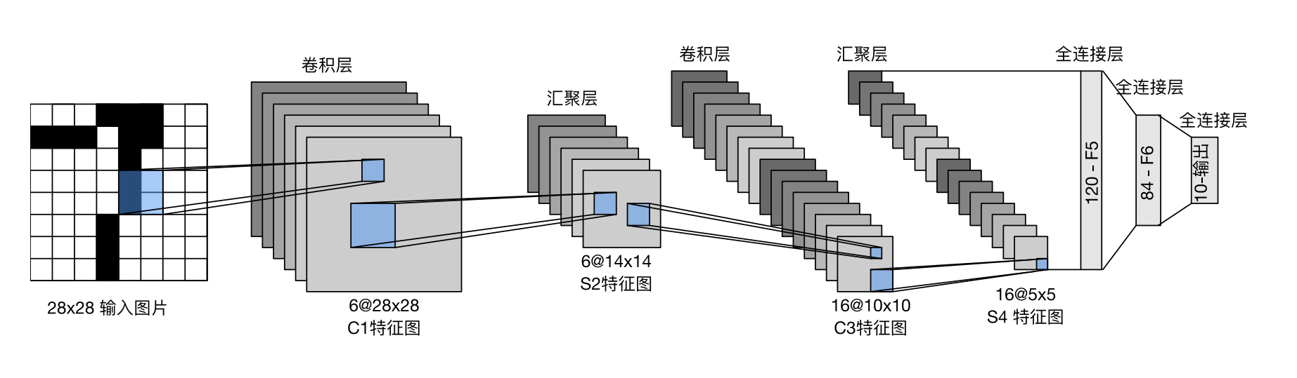
6.3 LeNet-5

现代卷积神经网络的奠基之作。正是其首次引入卷积层和池化层这两个核心组件，构建了现代 CNN 的基本结构范式。

总体来看，LeNet（LeNet‐5）由两个部分组成：

卷积编码器：由两个卷积块构成。
全连接层密集块：由三个全连接层构成。

其结构图如下图所示（D2L 图6.6.1）：

接下来准备做代码复现，不过这里的实现和原来的模型略有不同：

激活函数使用 ReLU，而不是 sigmoid 或 tanh。
LeNet-5 的标准输入为，但 MNIST 图片的尺寸是，简单起见，直接在 transfrom 里加一个 Resize((32, 32))。

transform = transforms.Compose([
    transforms.Resize((32, 32)),
    transforms.ToTensor(),
])

train_data = torchvision.datasets.MNIST(root = './mnist', train = True, transform = transform, download = True)
test_data = torchvision.datasets.MNIST(root = './mnist', train = False, transform = transform, download = True)

train_loader = torch.utils.data.DataLoader(train_data, batch_size = BATCH_SIZE, shuffle = True)
test_loader = torch.utils.data.DataLoader(test_data, batch_size = BATCH_SIZE, shuffle = False)

class LeNet5(nn.Module):
    def __init__(self):
        super(LeNet5, self).__init__()

        self.get_feature = nn.Sequential(
            # C1: 卷积层 (1通道 -> 6通道, 卷积核 5x5)
            # Input: 32x32 -> Output: 28x28
            nn.Conv2d(in_channels = 1, out_channels = 6, kernel_size = 5),
            nn.ReLU(), # Sigmoid 太菜了，换 ReLU
            
            # S2: 下采样 (AvgPool)
            # Input: 28x28 -> Output: 14x14
            nn.AvgPool2d(kernel_size = 2, stride = 2),
            
            # C3: 卷积层 (6通道 -> 16通道, 卷积核 5x5)
            # Input: 14x14 -> Output: 10x10
            nn.Conv2d(in_channels = 6, out_channels = 16, kernel_size = 5),
            nn.ReLU(),
            
            # S4: 下采样 (AvgPool)
            # Input: 10x10 -> Output: 5x5
            nn.AvgPool2d(kernel_size = 2, stride = 2)
        )

        self.classify = nn.Sequential(
            nn.Flatten(), # 展平: 16 * 5 * 5 = 400
            # 120-F5: 全连接层
            nn.Linear(in_features = 16 * 5 * 5, out_features = 120),
            nn.ReLU(),
            
            # 84-F6: 全连接层
            nn.Linear(in_features = 120, out_features = 84),
            nn.ReLU(),
            
            # 10-输出
            nn.Linear(in_features = 84, out_features = 10)
        )

    def forward(self, x):
        x = self.get_feature(x)
        x = self.classify(x)
        return x

model = LeNet5().to(DEVICE)

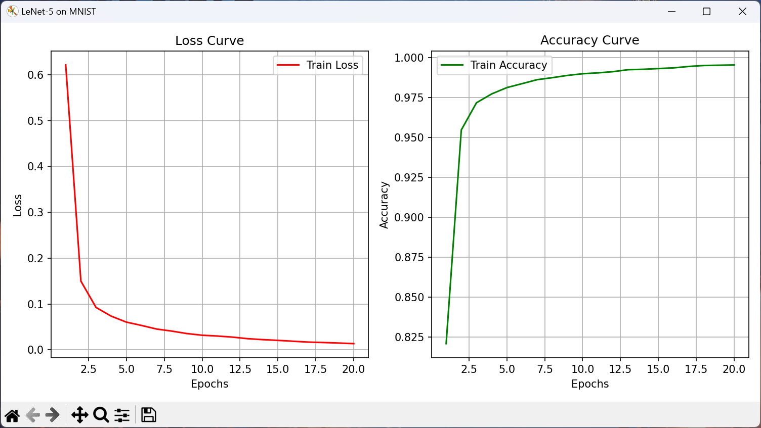
训练输出：

Device: cuda
Batch Size: 256
Learning Rate: 0.001
=============== Training Process ===============
Epoch 1/20 | Loss: 0.6215 | Train Acc: 0.8208
Epoch 2/20 | Loss: 0.1499 | Train Acc: 0.9547
Epoch 3/20 | Loss: 0.0924 | Train Acc: 0.9718
Epoch 4/20 | Loss: 0.0734 | Train Acc: 0.9773
Epoch 5/20 | Loss: 0.0604 | Train Acc: 0.9813
Epoch 6/20 | Loss: 0.0530 | Train Acc: 0.9838
Epoch 7/20 | Loss: 0.0452 | Train Acc: 0.9862
Epoch 8/20 | Loss: 0.0407 | Train Acc: 0.9875
Epoch 9/20 | Loss: 0.0354 | Train Acc: 0.9889
Epoch 10/20 | Loss: 0.0317 | Train Acc: 0.9900
Epoch 11/20 | Loss: 0.0300 | Train Acc: 0.9905
Epoch 12/20 | Loss: 0.0276 | Train Acc: 0.9913
Epoch 13/20 | Loss: 0.0242 | Train Acc: 0.9925
Epoch 14/20 | Loss: 0.0221 | Train Acc: 0.9928
Epoch 15/20 | Loss: 0.0205 | Train Acc: 0.9932
Epoch 16/20 | Loss: 0.0186 | Train Acc: 0.9937
Epoch 17/20 | Loss: 0.0168 | Train Acc: 0.9946
Epoch 18/20 | Loss: 0.0159 | Train Acc: 0.9951
Epoch 19/20 | Loss: 0.0147 | Train Acc: 0.9953
Epoch 20/20 | Loss: 0.0134 | Train Acc: 0.9955
=============== Time Usage: 138s ===============
Test Accuracy: 0.9904

非常强大。

7. 现代卷积神经网络

书上介绍的网络有 AlexNet、VGG、NiN、GoogLeNet、ResNet、DenseNet，这里不按书上的来。

7.1 VGG

见 VGG网络学习笔记。

7.2 GoogLeNet

见 GoogLeNet 学习笔记。

7.3 Batch Normalization

咕咕咕

7.4 ResNet

见 ResNet 学习笔记。

7.5 MobileNet

咕咕咕

7.6 R-CNN

咕咕咕

Loading...

1. 引言

2. 预备知识

3. 线性神经网络

3.1 线性回归

线性问题模型

损失函数

平方误差

均方误差 (Mean Squared Error, MSE)：

平均绝对误差（Mean Absolute Error, MAE）：

Huber Loss

目标

解析解

随机梯度下降（Stochastic Gradient Descent, SGD）

训练步骤

模型预测

3.2 线性回归代码实现

3.3 softmax 回归

分类问题模型

softmax 运算

交叉熵损失

3.4 softmax 回归 实现 Fashion-MNIST 分类

4. 多层感知机

4.1 隐藏层

4.2 激活函数

4.3 实现 MLP

4.4 咕咕本章其它部分

5. 深度学习计算

5.1 层和块

5.2 重构 MLP

5.3 save & load

SL Tensor

Save

Load

SL Model

Save

Load

SL Optimizer

Save

Load

5.4 咕咕本章其它部分

6. 卷积神经网络

6.1 从全连接到卷积

卷积层

通道

输出大小计算

多输入通道

多输出通道

卷积

6.2 池化层（pooling layer）

多通道

6.3 LeNet-5

7. 现代卷积神经网络

7.1 VGG

7.2 GoogLeNet

7.3 Batch Normalization

7.4 ResNet

7.5 MobileNet

7.6 R-CNN

3.4 softmax 回归实现 Fashion-MNIST 分类